Perception of sound
14 Interpreting graphs
Sound graphs
When you record sound using a microphone, vibrations of the air turn into electrical signals. The resulting electrical signal can be recorded, graphed and analyzed. While you cannot directly read sensations like pitch and loudness from a graph, you can make many reasonable inferences how a recording sounds by examining graphs.
Time domain graphs
In most sound recording software, time domain graphs are the default display. Most programs show ten seconds or more of the time domain plot on the screen. With so much time shown on one graph, you can usually see how the loudness is changing. To “read loudness” off a time domain sound graphs, focus on the height of the trace. Large amplitude indicates loud moments in the recording. Small amplitude indicates quiet sound. If amplitude increases from left to right, sound is probably getting louder over time (a crescendo in musician-speak).
If you zoom in on the time axis enough, information about the vibrations becomes visible. You can tell pitch from noise. You can measure the fundamental frequency (and therefore say something about pitch). You can make guesses about the spectral content. In practice, most sound engineers and scientists do not use the time domain graphs this way- it’s too time consuming. Other graphs (FFTs and spectrograms) yield frequency information faster and easier.
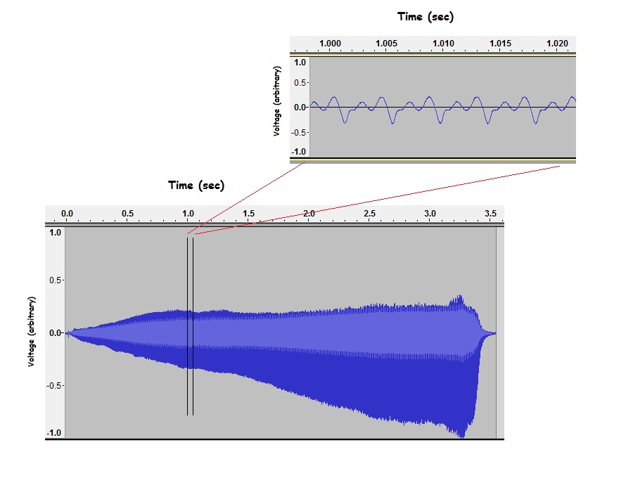
From the zoomed out graph above, you can tell that this Mystery Sound starts nearly silent and gets steadily louder for about 3.3 seconds. The sound then drops to near-silence in about 0.2 seconds. Zooming in near t=1.0 second reveals more info. About 1.0 seconds into the recording, the vibration is periodic and complex- what we hear at this point is pitched sound with at least a few overtones. You can estimate the fundamental frequency- read the fundamental period from the graph and apply [latex]f = \dfrac{1} {\tau}[/latex]. During the time frame shown in the inset, the period is roughly 0.0042 s, so the fundamental frequency is roughly 240 Hz. To find out how pitch is changing over the entire recording, you would have to look at several more zoomed-in sections of the graph- a tedious process.
Frequency domain graphs
Most audio recording programs allow you to make spectrum plots- either in real time, or by selecting a section of the recording. FFTs give you details about the spectral content of a short snapshot of the sound. You can tell pitched sound from noise. You can tell which frequencies are most dominant in a complex sound. You can sometimes identify different components of a sound that is a mixture of noise and pitched sound. FFTs are snapshots- that limits their usefulness. In practice, FFTs are only useful when you need detailed spectral information about a sound that isn’t changing much or you need detailed spectral information at a particular point in the recording.
The FFT below was taken from the recording of the Mystery Sound shown above. The FFT is taken about 1.0 seconds into the recording- during the same short time window as the inset on the Mystery Sound time domain graph.
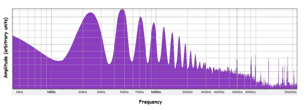
The FFT mostly confirms what we already know- about 1.0 second into the recording, the Mystery Sound has a fundamental of about 240 Hz and many overtones. The FFT does reveal additional details about the overtones- what the frequencies are and what the relative amplitudes are. For instance, the highest amplitude peak on the FFT is not the fundamental.
Spectrograms
Spectrograms are most useful for identifying how frequency and spectral content change over time. Spectrograms, for instance, are widely used for analyzing animal sounds, from human speech to bird calls.
Once you get the knack of reading them, spectrograms show lots of information about a recording quickly. Keep in mind that frequency is graph along the vertical axis and time is along the horizontal. In many ways, reading a spectrogram is a lot like reading music. Horizontal positioning indicates when a sound occurs. Vertical positioning indicates the frequency. Vertically aligned marks indicate sounds that happen simultaneously.
It’s easy to tell noise from pitched sound. Spectrograms of pitched sounds have distinct, narrow stripes. Spectrograms of noise lack distinct bands. Spectrograms of complex tones show multiple narrow bands, one above another. (The band lowest on the graph is the fundamental). On a spectrogram, events are shown in chronological order- earliest sounds are at the left end of the graph. Stripes that sweep up and to the right show sounds that are increasing in pitch. Horizontal stripes indicate a constant tone. Vertical bands indicate bursts of noise. Spectrograms show amplitude (fainter marks indicate quieter sound), but it’s often hard to see. Un-zoomed time domain graphs show amplitude changes far more clearly.
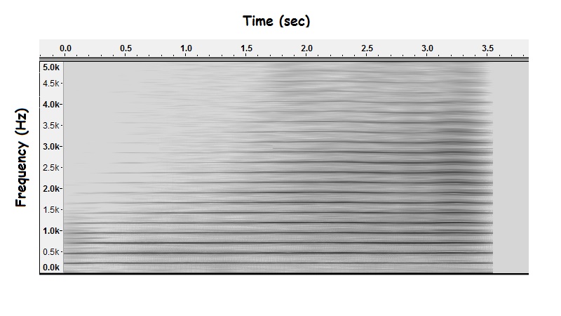
Above is a spectrogram of the Mystery Sound. Stripes show that the sound is pitched- not just at a point 1.0 seconds into the recording, but throughout the entire recording. The existence of stacked stripes confirms the existence of overtones. The fact that the stripes are horizontal reveals something new- the pitch is the same throughout the entire 3.5 second recording.
Notice that the stripes at higher frequencies are barely visible early in the recording. During the first 0.2 seconds of the sound, the amplitude of overtones above 1 kHz is very small or zero. As the sound goes on, the amplitude of the higher overtones increases.
Mystery Sound Revealed
The Mystery Sound is a trombone player playing a single note [latex](B \flat 3)[/latex] for roughly 3.3 seconds, starting off softly and getting louder. At the end of the note, the trombone player stops. There is a short delay (about 0.2 seconds) between when the trombone player stops playing and when the sound actually dies out.
Image credits
- Time domain graph of a Mystery Sound. Inset shows a zoomed-in portion of the graph. Created by Abbott using Audacity.
- FFT of a short sample of Mystery Sound, taken about 1.0 seconds into the recording. Created by Abbott using Audacity.
- Spectrogram of Mystery Sound. Created by Abbott using Audacity.
